Update: The self-driving RC car project now has a GitHub repository! You can find all the code that I end up writing in this repo. There are detailed instructions in the readme for you to be able to use all the code.
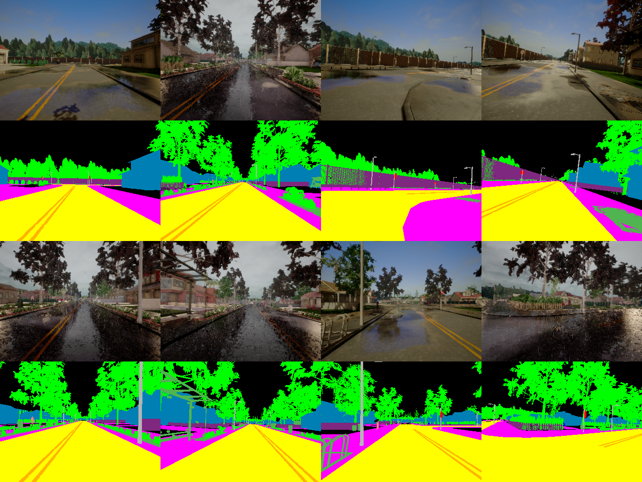
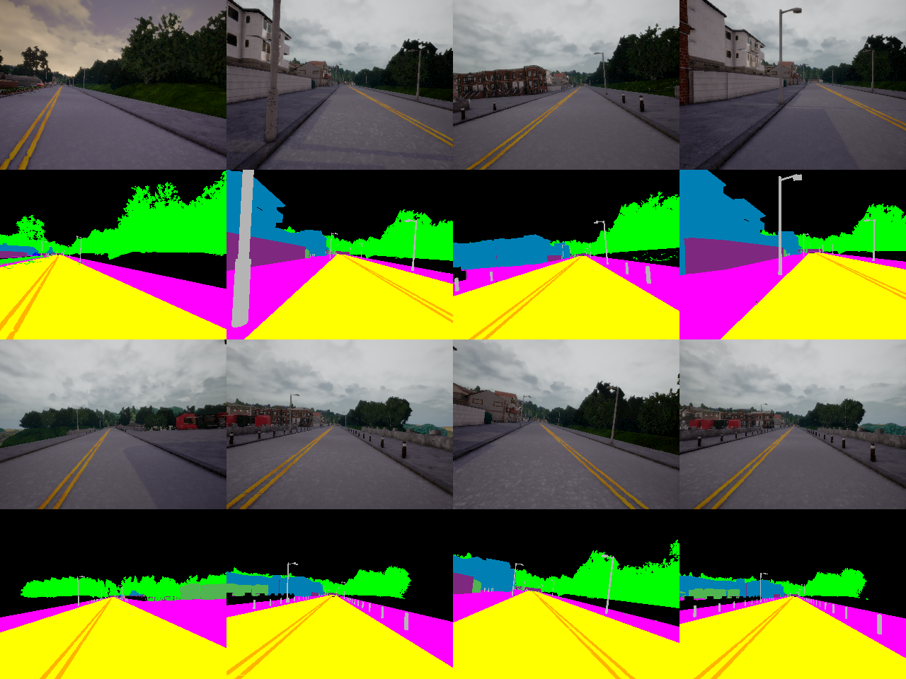
Getting data out of the CARLA simulator is not as trivial as it seems; it really deserves an entire blog post. Here are some images to whet your apetite for what’s in the rest of this post (these images will make sense to you by the end of the post):

If you recall from the first blog post in this series, one of the biggest reasons I chose CARLA is that it can generate ground truth data for semantic segmentation, which in turn makes it much easier to detect not only lanes but also other vehicles and objects in the camera feed, and it has a lot of weather and lighting conditions, and a variety of vehicles and roads.
While I had promised to use CARLA version 0.8.2 in the previous post, I ended up using version 0.8.4 instead, because:
- version 0.8.4 has two towns whereas version 0.8.2 has only one
- there are two wheelers in version 0.8.4 in addition to four-wheelers
- it has a pre-built binary for Windows, unlike version 0.9.2 (the latest and greatest) which does not. I actually tried to build it from source, but as of the time of writing, it is not possible to build the Python client libraries on Windows for that version (look at this issue), so I had to give up on it (after three whole days of trying).
The following is my effort to make CARLA more accessible, because the documentation for the simulator (and especially the Python API) is sparse to say the least, even for the stable version (they are trying to do a better job for the latest version, but that version is riddled with bugs right now).
Note that if you don’t have a computer with a dedicated graphics card, then you will most certainly not be able to run CARLA, or at least get reasonable framerates while collecting data. In that case, you can ask me in the comments for the data that I have collected and I can share that with you.
CARLA Basics
The basic idea is that the CARLA simulator itself acts as a server and waits for a client to connect. A
Python process connects to it as a client. The client sends commands to the server to control both the
car and other parameters like weather, starting new episodes, etc. The server (i.e., the simulator) sends
measurements and images back to the Python process. The Python client process can then print the received
data, process it, write it to disk, etc. By default all the communication between the client and the server
happen on TCP ports 2000, 2001 and 2002. The messages sent and received on these ports is explained
here, but it is not very important to
understand everything over there, as most of the client-server communication is abstracted by the carla
module in the PythonClient directory.
Getting Data
As discussed in the previous post, I do not want to train an end-to-end neural network because I want to stay away from unpredictable black boxes. Instead, I want to use more predictable algorithms that can be understood and explained, and whose behavior can be extrapolated reliably. The first step in doing that, of course, is to get images of driving. And the task of finding lanes and other obstacles in our path can be greatly simplified by using a neural network capable of semantic segmentation, because traditional computer vision techniques can’t recognize lane lines, cars, etc. with as much generalization as deep neural networks, so we can delegate that task to a semantic segmentation neural network and then build algorithms on top of that. So we also want to get semantic segmentation ground truth to train the neural network with.
It would’ve been really helpful if CARLA had documentation for their Python API for versions 0.8.x, but
all they have for us are five example scripts in the PythonClient directory and accompanying information
on the documentation website. We are supposed to figure out how to use CARLA by ourselves using that
information. While inconvenient, it is not impossible.
Since I wanted to drive the car manually and collect data, I found it easiest to modify the
manual_control.py file in the PythonClient directory. The final version,
manual_control_rgb_semseg.py
is in the official repository for this project. In order
to figure out how to save data, I referenced the client_example.py file in the PythonClient directory.
But turns out, the technique used in that script to save the data is awful. They are saving each image
(frame) to disk as a .png file as it is coming in. This is exactly how not to save data when you want
to keep up with a real-time task such as a running simulator, because writing to disk is a painfully slow
process and waiting for the Python client process to write to disk after each frame causes the framerate
to drop to about 3-4 fps at best. Hard disks and SSDs alike give the best write speeds if you try to
write a few large files at once rather than writing many small files. And storing data in RAM is way
faster than saving it on disk.
Finally, since I eventually want to train a neural network with the collected data, it would be really
convenient if all my collected data were stored in numpy arrays. Then I would not have to open thousands
of .png files and read them into memory. Storing and retrieving the data in bulk would also be very
easy because there would be no need to encode/decode from the PNG format, and besides, both opencv and
matplotlib work with numpy arrays under the hood, so it does not make visualization any harder. (What?
You want to use an image viewer? Use Jupyter Notebook instead. Like a real programmer.)
Saving Incoming Data Efficiently
You can criticize my software design decisions here, but my solution to all the aforementioned problems works perfectly and is quite extensible, if a little redundant in places. Here is an overview of my idea:
- The data will be stored in a large numpy array as it comes in. This is particularly convenient, because the data comes in as 32-bit integers that can be read as 8-bit integers to obtain BGRA images.
- The data is processed by type.
- Once the large numpy array (I call it a
bufferin the code) fills up, we can write it to disk and make a new, empty buffer. The disk write is neither nonblocking nor asynchronous, but it takes less than a second and happens after several minutes of uninterrupted gameplay, so overall framerate does not take a hit.
If you take a look at the file buffered_saver.py,
you will find a BufferedImageSaver class which does all the magic. Each BufferedImageSaver object
has a buffer (numpy array) where it stores the incoming data. Since the numpy array is in memory (RAM),
writing to it is very fast. Each instance also stores the sensor type associated with it to determine
what processing to apply to incoming data. The BufferedImageSaver.process_by_type method takes in
the raw data provided by the simulator each frame. If the sensor is an RGB camera, it does not do
anything. But if it is semantic segmentation ground truth, then it removes all but the red channel,
because it is the only channel with any information (as explained
here).
If the sensor type happens to be a depth camera, it converts the information in the three channels into
a single “channel” of floating point data, applying processing similar to
this.
After every frame, the BufferedImageSaver.add_image method is called with the raw sensor data, which either
stores the data in the buffer, or if the buffer is full, saves the buffer to disk, resets the buffer, and
then stores the incoming data. You do not need to understand all the code, and the API is pretty simple.
You can look here
to see how to create a BufferedImageSaver object. And
this
is how to add an image to a BufferedImageSaver object. There is really nothing more to the API.
This solves all the problems that I enumerated in the previous section.
Running the Simulation and Saving the Data
This is a great time to read the section of the readme titled CARLA Simulator Scripts. It explains exactly how to run the simulator and start collecting data. I will go over a few important points here.
It is essential that you start the simulator in
fixed time-step mode.
This means you need to use the -benchmark flag and provide an fps=<framerate> argument (where
<framerate> is some framerate that is reasonable given your hardware) while starting the simulator,
like this:
# on Linux
./CarlaUE4.sh -carla-server -benchmark -fps=<framerate>

# on Windows
CarlaUE4.exe -carla-server -benchmark -fps=<framerate>
And the following line must be present in the CarlaSettings object in the client code in order to
enable synchronous mode:
settings = CarlaSettings()
settings.set(SynchronousMode=True)
as you can see here.
Basically, running in synchronous mode makes sure that the Python client is able to keep up with all the data that the simulator bombards it with. When not running in synchronous mode, the simulator sends data (sensor measurements and images) as soon as they are rendered, and if the Python client is not able to capture the data right away, it may be lost forever once the next packet arrives. This actually led to the semantic segmentation ground truth not matching the camera images, as you can see below:

At first glance, you may not notice any problems, but if you look carefully at the second image from the left, you will notice how the pole is in a different place in the semantic segmentation ground truth compared to the raw image. Look here for more examples of this. What is happening in these cases is that the Python client is not being able to read the incoming images fast enough, and is, in a sense, dropping frames. This can be potentially very detrimental and might keep our semantic segmentation model from converging.
Running in synchronous mode forces the simulator to wait for a control signal from the Python client before sending the next packet of data. This is how to send a control message:
client.send_control(control)
as you can see here.
Since we are sending the control signal after storing the sensor data, we are guaranteed not to drop any frames, and we get semantic segmentation ground-truth that is perfectly aligned with the camera images:

As explained in the readme, if you start the Python client with the following command:
python3 manual_control_rgb_semseg.py --images-to-disk --location=<save_location>
the data will be stored in <save_location>. But these data are massive numpy arrays (.npy files),
so it is best to use a Jupyter Notebook to interactively visualize them to make sure that there are no
problems with the data. (I actually discovered the problem of semantic segmentation ground truth not
being synchronized with camera images only after visualizing the collected data in a notebook!)
Verifying the Saved Data
I have included a Jupyter Notebook called
verify_collected_data.ipynb
in the CARLA_simulator_scripts
directory which will allow you to painlessly visualize the saved data.
The visualization process is quite simple: we first load the numpy arrays from disk into memory.
Now, I lied to you when I said that the camera captures RGB images. It actually saves images in BGR
format, because Unreal Engine uses the BGRA format for images (it is trivial to get rid of the alpha
channel but I did not bother to convert from BGR to RGB while saving the numpy arrays in
buffered_saver.py
because neural networks don’t care either way). So we use opencv to convert the images from BGR to RGB
in the notebook:
img = cv2.cvtColor(img, cv2.COLOR_BGR2RGB)
As for the semantic segmentation ground truth arrays, we need to convert the categorical indices (listed
here) into
actual colors. It can be done easily by passing a
categorical (qualitative) color map
to the cmap argument to the function matplotlib.pyplot.imshow as follows:
plt.imshow(display_array[:, :, 0], cmap='tab20', aspect='auto')
Passing the value 'auto' to the aspect parameter indicates that we want the aspect ratio of the images
to be varied to fit the given axes. This makes the visualizations better in this case.
Below the visualizations is the code I used to generate the images in this blog post. Basically, I am
converting the categorical semantic segmentation ground truth to RGB using a custom color mapping function
map_semseg_colors which outputs an RGB image that can then be saved using the pillow (PIL) library.
You will probably not need to use that code.
Going Forward
Getting images from the simulator took much longer than I had originally anticipated (partly because I wasted three days trying to build CARLA version 0.9.2 from source on Windows). But going forward, finding lanes should not be that difficult, as it is almost trivial to find lanes from semantic segmentation output, and we only have to fit the detected lanes, which is much easier than finding the lanes themselves. I will make a post about that in the coming days, so stay tuned!
If you have any questions, comments, criticism, or suggestions, feel free to leave them below. If you know someone who is interested in content like this, please share this article with them. Once again, the official repository for this project is here, and please let me know if you want the data I have collected. The only reason the data is not freely available right now is that I am not sure how to host a few gigabytes of data online for free.